| Myth | Reality |
|---|---|
| A model that passed offline evaluation will keep performing the same way in production. | Input distributions and real-world relationships shift continuously; a model frozen in time will drift away from reality regardless of how good its original evaluation looked. |
| If a model is failing, an error or crash will alert the team. | Most production model failures are silent: the model keeps returning confident, well-formed predictions that are simply wrong, with no exception thrown anywhere. |
| Monitoring accuracy is enough. | Ground-truth labels are often delayed by days, weeks, or never arrive at all, so accuracy-only monitoring misses degradation until it is far too late to matter. |
| One dashboard threshold covers every failure mode. | Data drift, concept drift, and training-serving skew each require different detection techniques and different response playbooks. |
Why Production Models Fail Quietly
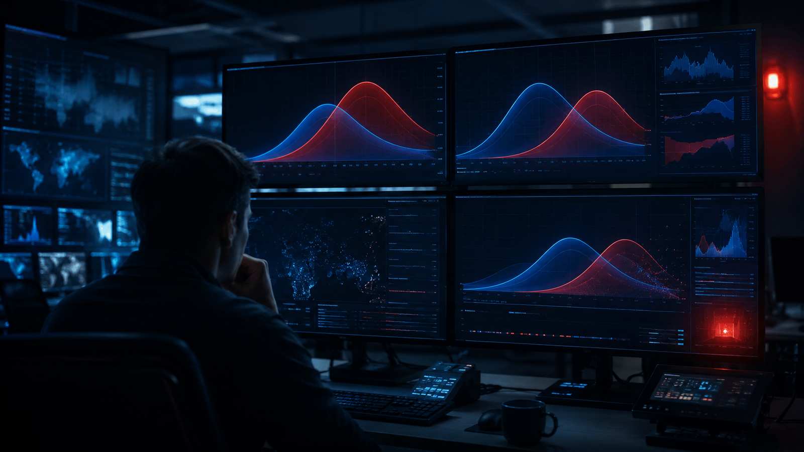
Machine learning models do not usually fail the way traditional software fails. A web server that crashes throws a stack trace. A model that has quietly drifted away from the distribution it was trained on keeps returning confident, well-formatted predictions, just wrong ones. Nothing crashes. No error budget gets consumed. The only signal is a slow, often invisible decline in business outcomes that frequently gets attributed to something else entirely, seasonality, a marketing change, a competitor, before anyone thinks to check the model itself.
This is the core argument for treating model monitoring as a first-class discipline rather than an afterthought bolted onto a deployment pipeline. AI systems rarely fail loudly; they degrade quietly, and most teams do not notice until a stakeholder complains, by which point the model may have been wrong for weeks or months. The goal of a monitoring program is to convert that silent failure into a detectable, actionable signal long before a human notices something feels off.
The Four Distinct Failure Modes
Not all production model degradation is the same problem, and treating it as one undifferentiated bucket called “the model is broken” makes diagnosis much harder than it needs to be. There are four distinct failure modes, each with its own detection approach.
| Failure mode | What changes | Typical cause | Detection approach |
|---|---|---|---|
| Data drift | Input feature distributions shift over time | User behavior change, new market segment, upstream data source change | Population Stability Index, KL divergence on feature distributions |
| Concept drift | The relationship between inputs and the true outcome changes | Real-world dynamics change, e.g. fraud patterns evolve, consumer preferences shift | Tracking prediction accuracy against delayed ground truth, performance decay curves |
| Training-serving skew | Feature values differ between training and live serving code paths | Divergent pipelines, different null handling, different aggregation windows | Comparing offline-computed and online-computed feature values directly, shadow deployments |
| Silent label-free degradation | Model quality declines with no ground truth available to measure it against | Long label delay, no labels at all, feedback loops removed | Prediction distribution drift, confidence score monitoring, proxy metrics |
Data drift and concept drift are frequently confused, but they are not the same problem. Data drift means the inputs a model sees have changed, the distribution of transaction amounts, the mix of user demographics, the range of sensor readings, while the underlying relationship between those inputs and the correct output has stayed the same. Concept drift means the relationship itself has changed: a fraud model’s features look the same, but what predicts fraud has evolved because fraudsters have adapted their tactics. A model can experience one without the other, and mistaking one for the other leads to the wrong fix, retraining on more of the same data does nothing for concept drift if the underlying labels being used to retrain are already stale.
Training-serving skew deserves special mention because it is the failure mode most directly tied to engineering practice rather than the external world changing. It happens when the feature computation logic used during training diverges from the logic used during live inference, and a well-implemented feature store, discussed later in this piece, is one of the more effective structural defenses against this exact failure mode.
Detection Techniques That Actually Work
Population Stability Index, commonly abbreviated PSI, is one of the most widely used metrics for detecting data drift. PSI quantifies how much a feature’s distribution has shifted compared to a reference distribution, typically the distribution seen during training, and it has the practical advantage of being symmetric, meaning it treats a shift from A to B the same as a shift from B to A. This makes it easy to set stable alert thresholds that do not need constant recalibration.
KL divergence, short for Kullback-Leibler divergence, is a related statistical distance measure that also quantifies how different one probability distribution is from another. Unlike PSI, KL divergence is not symmetric, which can make it a better fit for cases where the direction of the shift genuinely matters, but a worse fit for simple dashboard alerting where teams want one number that behaves predictably in both directions.
Shadow deployments provide a different kind of signal entirely. Rather than comparing distributions statistically, a shadow deployment runs a new or updated model alongside the current production model, feeding it the same live traffic but withholding its predictions from actually affecting users. This lets teams directly compare a candidate model’s behavior against the incumbent’s on real, current data before any live decision depends on it, catching training-serving skew and unexpected behavior changes that offline evaluation alone would miss.
Figure: The Layered Monitoring Stack
A reliable monitoring setup stacks four layers: data quality checks at the input boundary, drift signals (PSI, KL divergence) on features and predictions, performance signals against delayed ground truth where available, and a documented response playbook that defines who gets paged and what they do next.
The Tooling Landscape
A handful of platforms have become the default choices for teams building out model monitoring in 2026, each with a different center of gravity.
| Tool | Strength | Best fit |
|---|---|---|
| Evidently AI | Over 100 built-in metrics, open-source core, interactive reports | Teams wanting a flexible, self-hostable monitoring layer integrated into existing MLOps pipelines |
| Arize | Unified platform spanning the full model lifecycle, strong LLM and agent observability | Organizations running both classic ML and newer LLM-based systems side by side |
| WhyLabs | Privacy-oriented, works from statistical profiles rather than raw data | Regulated environments where raw data cannot leave a security boundary |
| Fiddler | Deep explainability, fairness monitoring, governance features | Teams with strong responsible-AI and compliance requirements |
The practical distinction that matters most when choosing between them is less about raw metric count and more about where your organization’s actual constraint sits. If regulatory or security policy prevents raw data from leaving your environment, WhyLabs’ profile-based approach solves a problem that other tools do not directly address. If your primary risk is a biased or non-compliant model decision rather than a drifted one, Fiddler’s fairness and governance tooling is purpose-built for that. If you are already running LLM-based systems alongside traditional models, Arize’s broader lifecycle coverage avoids running two separate monitoring stacks. Evidently AI’s open-source core also makes it a common starting point for teams that want to prototype a monitoring layer before committing budget to a managed platform, since its metrics library can be adopted incrementally alongside an existing pipeline rather than requiring a full platform migration up front.
Building a Layered Monitoring Setup
A monitoring program that only checks one layer will eventually miss a failure that another layer would have caught. The pattern that has proven durable across teams is a four-layer stack, ordered roughly by how early each layer can catch a problem.
- Data quality checks. Schema validation, null rate checks, range checks, and freshness checks at the point data enters the pipeline. These catch the crudest problems, a broken upstream feed, a null column, before they ever reach a model.
- Drift signals. PSI or KL divergence computed on both input features and model outputs, alerting when a distribution moves meaningfully away from its training-time reference.
- Performance signals. Direct accuracy, precision, recall, or business-metric tracking wherever ground truth eventually becomes available, even if delayed.
- A response playbook. A documented, rehearsed process defining who gets paged when an alert fires, what the first three diagnostic steps are, and under what conditions the model gets rolled back versus retrained.
The fourth layer is the one teams skip most often, and it is arguably the one that determines whether the first three layers actually matter. A drift alert that fires into a channel nobody monitors, or that has no defined owner, produces exactly the same outcome as having no monitoring at all: silent failure, just with an ignored alert sitting in the history for the postmortem to reference later.
Handling Silent, Label-Free Degradation
The hardest of the four failure modes to monitor is the one where no ground truth is available at all, or where it arrives so late that direct accuracy tracking is useless for early detection. This is common in settings like long-cycle credit decisions, medical outcomes, or any prediction whose “correctness” is only knowable months later. In these cases, teams rely on proxy signals: monitoring the distribution of the model’s own predictions and confidence scores for unexpected shifts, using shadow models trained on more recent data to flag disagreement with the production model, and tracking upstream data drift as a leading indicator even without direct performance confirmation.
None of these proxies are as reliable as direct ground-truth accuracy tracking, and teams that rely on them exclusively should treat drift alerts as a prompt to investigate rather than definitive proof of degradation. The honest position is that label-free monitoring reduces the size of the blind spot; it does not eliminate it.
Common mistake
Teams set a single global drift threshold across every feature and every model, then either drown in false positives from naturally noisy features or miss real drift in low-variance features that should have tighter thresholds. Thresholds need to be set per feature based on its historical volatility, not applied uniformly.
What worked
Teams that paired automated drift alerts with a mandatory weekly review of the top five most-volatile features, rather than waiting purely for threshold breaches, caught slow concept drift that no single alert crossed a threshold for, because the trend across weeks was the actual signal, not any single data point.
Frequently Overlooked Details
- Reference window choiceThe baseline distribution PSI or KL divergence compares against matters enormously; using a stale training-time reference forever will eventually flag normal seasonal variation as drift.
- Prediction driftA change in the distribution of model outputs, even without confirmed ground truth, often serves as the earliest available leading indicator that something upstream has shifted.
- Alert fatigueOver-alerting on minor, expected fluctuations trains teams to ignore monitoring dashboards entirely, which defeats the purpose of having them.
- Feedback loop contaminationWhen a model’s own predictions influence the future data it is later evaluated against, performance metrics can look artificially stable while real-world accuracy quietly declines.
- Segment-level driftAggregate metrics can look healthy while a specific customer segment or geography experiences serious degradation that gets averaged away.
Designing Alert Thresholds That Hold Up
| Signal type | Typical alert trigger | Response urgency |
|---|---|---|
| PSI on a core feature | Above 0.2 sustained over multiple windows | Investigate within a business day |
| Prediction distribution shift | Significant deviation from rolling baseline | Investigate within hours if paired with a business-metric dip |
| Confirmed accuracy drop | Statistically significant decline against delayed ground truth | Immediate, treat as an incident |
| Training-serving skew detected in shadow deployment | Any material mismatch between offline and online feature values | Block deployment until resolved |
These thresholds are starting points, not universal constants; the right number for any given feature depends on its natural volatility, and a feature with high day-to-day variance under normal conditions needs a looser threshold than a feature that is normally extremely stable. Reviewing and recalibrating thresholds on a regular cadence, rather than setting them once at launch, is what keeps a monitoring system useful instead of becoming background noise.
Estimating the Cost of Undetected Drift
Teams that have never quantified the cost of silent failure tend to underinvest in monitoring, because the cost is diffuse and hard to attribute after the fact. A useful exercise is to estimate, even roughly, how many weeks a typical drift episode goes unnoticed under current practices, then multiply that by the daily cost of the affected decision, a fraud model missing a growing pattern, a recommendation model quietly serving worse suggestions, a credit model misjudging a shifted population. Even a rough estimate usually makes the case for a monitoring investment obvious, because the multiplication tends to dwarf the cost of the tooling and headcount needed to catch the problem in days rather than months.
This calculation also clarifies where to invest first. A model with a large blast radius, high transaction volume, high dollar value per decision, or safety-critical consequences deserves the tightest thresholds and the fastest response playbook, while a low-stakes internal model can reasonably tolerate a lighter monitoring footprint. Treating every model with identical monitoring rigor wastes attention on low-risk systems while under-monitoring the ones that matter most.
How Monitoring Fits Into the Broader ML Lifecycle
Model monitoring does not operate in isolation from the rest of the ML lifecycle. The features it watches are frequently served through a feature store, and a well-governed store makes skew detection dramatically easier, a connection explored in our feature stores explainer. The decision to retrain, roll back, or promote a new model based on monitoring signals should be validated with a properly designed experiment rather than a gut call, which is where our guide to A/B testing ML models becomes directly relevant. Monitoring for LLM-based systems introduces its own additional failure modes around retrieval quality, covered in our RAG architecture piece, and reproducibility practices that make a drifted model easy to roll back to a known-good state are covered in our reproducible ML guide. Broader organizational questions about who owns monitoring are addressed in our piece on building an ML platform team.
Glossary
- Data drift
- A change in the distribution of a model’s input features over time, without necessarily any change in the true relationship between inputs and outcomes.
- Concept drift
- A change in the underlying relationship between input features and the true outcome, meaning what the model learned is no longer valid even if the inputs look similar.
- Population Stability Index (PSI)
- A symmetric statistical measure quantifying how much a distribution has shifted relative to a reference distribution, commonly used to flag data drift.
- Shadow deployment
- A technique where a candidate model runs alongside the production model on live traffic without its predictions affecting real decisions, used to compare behavior safely before a full rollout.
- Prediction drift
- A shift in the distribution of a model’s own output predictions, often usable as an early warning signal even before ground-truth labels are available.
Key Takeaways
- Production models fail silently, continuing to produce confident, well-formed predictions that are simply wrong, with no error thrown anywhere.
- Data drift, concept drift, training-serving skew, and label-free degradation are four distinct failure modes requiring different detection techniques.
- Population Stability Index and KL divergence are the two most common statistical distance metrics for detecting distribution shifts.
- Shadow deployments let teams compare a candidate model against production on real traffic before it affects any live decision.
- Evidently AI, Arize, WhyLabs, and Fiddler each specialize around a different constraint: openness, LLM coverage, privacy, or governance.
- A layered monitoring stack, data quality, drift, performance, and a response playbook, catches failures that any single layer alone would miss.
- Alert thresholds must be set per feature based on natural volatility, not applied as one global number across the entire system.
FAQs
What is the difference between data drift and concept drift?
Data drift means the distribution of input features has changed while the true relationship between inputs and outcomes stays the same, whereas concept drift means that underlying relationship itself has changed, so the model’s learned patterns are no longer valid even if the inputs look familiar.
Why do production models fail without throwing errors?
Because a drifted or degraded model keeps producing syntactically valid, confident-looking predictions; there is no exception to catch, only a gradual decline in accuracy or business outcomes that often gets misattributed to other causes before anyone checks the model itself.
What is the Population Stability Index used for?
PSI quantifies how much a feature’s current distribution has shifted compared to a reference distribution, typically the training distribution, and its symmetry makes it a practical, stable metric for setting automated drift alert thresholds.
How does a shadow deployment help catch training-serving skew?
A shadow deployment runs a candidate model on the same live traffic as production without affecting real decisions, allowing direct comparison of predictions and feature values computed through the live serving path against what training-time computation would have produced.
What should teams do when ground-truth labels are delayed or unavailable?
Rely on proxy signals such as prediction distribution shifts, confidence score changes, and upstream data drift as leading indicators, while treating these proxies as a prompt to investigate rather than definitive confirmation of degradation.
How is training-serving skew related to feature stores?
Training-serving skew is caused by divergent feature computation code paths between training and serving, and a feature store addresses this directly by putting one shared feature definition behind both, which is why monitoring and feature store design are closely linked practices.
Why does alert fatigue undermine model monitoring?
When thresholds are too tight or applied uniformly across features with different natural volatility, teams get flooded with false alerts and eventually learn to ignore the monitoring dashboard entirely, which recreates the exact silent-failure risk monitoring was meant to prevent.
Is monitoring accuracy alone sufficient for production models?
No, because ground-truth labels needed to compute accuracy are frequently delayed by days or weeks, or never arrive at all, so accuracy-only monitoring misses the earlier warning signs that drift-based and data-quality layers are specifically designed to catch.
- Arize AI, Population Stability Index (PSI): What You Need To Know
- Arize AI, KL Divergence: When To Use Kullback-Leibler Divergence
- Fiddler AI Blog, Measuring Data Drift with the Population Stability Index
- N-iX, AI Observability Tools: How Enterprises Monitor Models
- Uplatz Blog, A Technical Leader’s Comparative Analysis of AI Observability Platforms: Evidently AI, Arize AI, and Fiddler AI
- InsightFinder, How Model Drift is Sabotaging Production AI Systems
- Medium, Comprehensive Comparison of ML Model Monitoring Tools: Evidently AI, Alibi Detect, NannyML, WhyLabs, and Fiddler AI