Predicting the future has been humanity’s obsession for millennia. Whether it is a farmer looking at the sky to save a harvest or a trader analyzing a ticker tape to secure a profit, the fundamental need remains the same: using past data to anticipate future states. Today, this age-old pursuit has evolved into the sophisticated field of time-series forecasting. While traditional statistical methods have served us well for decades, the explosion of big data has ushered in a new era dominated by deep learning for time-series forecasting.
This guide provides an extensive exploration of how deep neural networks are revolutionizing forecasting in two of the most data-rich and high-stakes industries: finance and weather. We will dissect the architectures that make this possible, explore the unique challenges of each domain, and provide a roadmap for understanding how these powerful models work in practice.
Key Takeaways
- Beyond Linear Models: Deep learning captures non-linear dependencies and complex patterns that traditional models like ARIMA often miss.
- Architecture Evolution: The field has moved from simple Recurrent Neural Networks (RNNs) to Long Short-Term Memory (LSTMs) and now to powerful Transformer-based models.
- Domain Specificity: While the underlying tech is similar, finance deals with high noise and behavioral psychology, whereas weather deals with physical laws and spatial dimensions.
- Data is King: Success depends heavily on preprocessing—handling missing values, stationarity, and normalization is critical.
- Hybrid Approaches: The most robust systems often combine deep learning with domain-specific knowledge (physics-informed AI or financial theory).
Who This Is For (And Who It Isn’t)
This guide is for:
- Data scientists and machine learning engineers looking to specialize in temporal data.
- Financial analysts and quants curious about the “black box” algorithms driving modern trading.
- Meteorologists and environmental scientists interested in data-driven alternatives to Numerical Weather Prediction (NWP).
- Tech-savvy business leaders who need to understand the capabilities and limitations of AI forecasting.
This guide is not:
- A surface-level news article about “AI hype.”
- A mathematical proof of backpropagation (though we discuss the mechanisms conceptually).
- A get-rich-quick guide for stock trading.
1. The Fundamentals of Time-Series Forecasting
Before diving into neural networks, we must ground ourselves in the basics. A time series is a sequence of data points collected or recorded at specific time intervals. Unlike standard regression problems where data points are often independent, time-series data possesses a temporal ordering that is sacrosanct—shuffling the data destroys its meaning.
Univariate vs. Multivariate Analysis
In its simplest form, forecasting involves univariate data: predicting the future value of a single variable (e.g., Bitcoin price) based solely on its own history. However, deep learning shines most brightly in multivariate scenarios, where the model considers multiple influencing variables simultaneously.
- Finance Example: Predicting a stock price using not just its past price, but also trading volume, interest rates, and sentiment scores from news headlines.
- Weather Example: Predicting temperature using past temperature, humidity, wind speed, and atmospheric pressure.
The Shift from Statistical to Deep Learning
For decades, the gold standard was statistical models like ARIMA (Auto-Regressive Integrated Moving Average) and GARCH (Generalized AutoRegressive Conditional Heteroskedasticity). These models are interpretable and effective for simple, stable datasets. However, they struggle with:
- High Dimensionality: Handling thousands of input features.
- Non-Linearity: capturing complex, chaotic relationships.
- Unstructured Data: Incorporating text (news) or images (satellite maps) into the prediction.
Deep learning bridges these gaps by learning feature representations directly from raw data, automating the complex feature engineering that statistical approaches require.
2. Core Architectures: The Engines of Prediction
To understand how deep learning forecasts the weather or stock prices, we must look under the hood at the neural architectures designed to handle sequential data.
Recurrent Neural Networks (RNNs)
Standard feedforward neural networks assume inputs are independent. RNNs introduced the concept of “memory” by looping the output of a neuron back into itself. This allows the network to maintain a hidden state containing information about previous inputs.
While revolutionary, basic RNNs suffered from the “vanishing gradient problem.” When training on long sequences—like daily temperature readings over ten years—the network would “forget” early data points as the error signals diluted during backpropagation.
Long Short-Term Memory (LSTMs) and GRUs
The LSTM was designed specifically to solve the memory limits of RNNs. It introduces a complex cell structure with three “gates”:
- Forget Gate: Decides what information from the previous state is irrelevant and should be discarded.
- Input Gate: Decides what new information is relevant and should be stored.
- Output Gate: Determines what the next hidden state should be.
This architecture allows LSTMs to capture long-term dependencies, such as a seasonal weather pattern that repeats annually or a long-term economic cycle in finance. A simplified variant, the Gated Recurrent Unit (GRU), combines some of these gates to achieve similar performance with lower computational cost, making it popular for real-time applications.
Convolutional Neural Networks (CNNs) for Time Series
Originally built for image recognition, 1D-CNNs (one-dimensional convolutional neural networks) have proven surprisingly effective for time series. Instead of scanning an image for edges, the convolution filter slides over the timeline to detect local patterns—such as a sudden “crash” pattern in a stock chart or a “front” in weather data.
- Why use them? They are incredibly fast to train compared to RNNs and are excellent at noise filtering.
- Dilated Convolutions: By skipping steps (dilation), these networks can expand their “receptive field” to see long histories without massive computational bloat.
Transformers and Attention Mechanisms
The current state-of-the-art in deep learning for time-series forecasting is dominated by Transformers. Originating in Natural Language Processing (NLP) with models like BERT and GPT, Transformers revolutionized sequential modeling by abandoning recurrence entirely.
Instead of processing data step-by-step (like an RNN), Transformers process the entire sequence simultaneously using Self-Attention mechanisms.
How Attention Works in Forecasting: Imagine trying to predict tomorrow’s weather. An LSTM reads yesterday, then the day before, sequentially. A Transformer looks at the last 30 days all at once and asks, “Which of these days are most relevant to tomorrow?” It might “attend” heavily to a day two weeks ago that had similar atmospheric pressure conditions, while ignoring a calm day yesterday.
Specific architectures like Informer, Autoformer, and Temporal Fusion Transformers (TFT) have been adapted explicitly for time series to handle the continuous nature of numerical data, distinguishing them from their language-model cousins.
3. Deep Learning in Finance: Taming the Chaos
Financial forecasting is often considered the “Holy Grail” of prediction. However, it is also notoriously difficult because financial markets are non-stationary (the rules change constantly) and stochastic (random).
The Unique Challenges of Finance
- Low Signal-to-Noise Ratio: Financial data is incredibly noisy. A stock price movement is often the result of random order flow rather than fundamental value shifts.
- Adversarial Environment: Unlike the weather, the market reacts to predictions. If a model predicts a stock will go up and a fund buys it, the price goes up immediately, essentially erasing the arbitrage opportunity.
- Regime Changes: A model trained during a bull market may fail spectacularly during a recession because the underlying statistical properties of the data have shifted.
Applications and Use Cases
1. Price and Volatility Prediction
While predicting the exact price of a stock is difficult, predicting volatility (how much the price will swing) is more feasible and highly valuable for pricing options and managing risk.
- Models used: Hybrid LSTM-CNN models are common here. The CNN extracts short-term trend features, while the LSTM captures the longer-term market sentiment.
2. Limit Order Book (LOB) Analysis
High-frequency trading (HFT) relies on analyzing the Limit Order Book—the list of buy and sell orders waiting to be executed. This data is massive and granular (tick-level data).
- Deep Learning approach: Deep learning models ingest millions of LOB updates per second to predict short-term price movements (microseconds ahead). Transformers are increasingly used here to identify complex liquidity patterns.
3. Algorithmic Trading and Portfolio Management
Reinforcement Learning (RL), a subset of deep learning, is used to train “agents” that make trading decisions. Instead of just predicting a price, the agent learns a policy: “If the LSTM predicts a 5% rise and volatility is low, BUY.”
- In practice: Large hedge funds use “Ensemble Learning,” where predictions from dozens of different deep learning models (some looking at news sentiment, others at price history) vote on a final decision.
4. Alternative Data Analysis
This is where deep learning creates the biggest edge.
- NLP: Analyzing earnings call transcripts and central bank statements using large language models (LLMs) to gauge sentiment.
- Computer Vision: Analyzing satellite imagery of retail parking lots to predict quarterly earnings for retail chains before they are announced.
4. Deep Learning in Weather: Modeling the Physics
Weather forecasting differs fundamentally from finance. It is governed by the laws of physics—specifically fluid dynamics and thermodynamics. However, the atmosphere is a “chaotic system,” meaning tiny errors in initial measurements grow exponentially over time (the Butterfly Effect).
The Evolution: From NWP to AI
Traditionally, weather is predicted using Numerical Weather Prediction (NWP). These are massive computer simulations that solve differential equations representing the atmosphere. They are precise but computationally expensive and slow; running a high-res global model can take hours on a supercomputer.
Deep Learning offers a paradigm shift: instead of solving equations, the AI learns the patterns of atmospheric evolution from historical data.
Applications and Use Cases
1. Precipitation Nowcasting
Nowcasting refers to short-term forecasting (0 to 6 hours ahead). This is critical for aviation, logistics, and flood warnings.
- The Deep Learning Edge: Traditional NWP is too slow for real-time updates. Deep learning models, specifically Generative Adversarial Networks (GANs) and ConvLSTMs (Convolutional LSTMs), treat weather radar maps as video frames. They predict the “next frames” of the radar video to show where the rain will move.
- Example: Google’s MetNet and DeepMind’s GraphCast have demonstrated the ability to predict precipitation at high resolution faster and often more accurately than physics-based models for short horizons.
2. Medium-Range Global Forecasting
For a long time, AI struggled to beat physics models at 7-10 day forecasts. This changed around 2023-2024.
- Graph Neural Networks (GNNs): The Earth is a sphere, not a flat grid. GNNs allow models to represent the atmosphere as a mesh or graph, handling the geometry of the globe correctly.
- Impact: Models like NVIDIA’s FourCastNet and Huawei’s Pangu-Weather can generate a 7-day global forecast in seconds on a single GPU, compared to hours on a cluster of CPUs for NWP.
3. Extreme Event Detection
Deep learning excels at pattern recognition, making it ideal for spotting the precursors to extreme events like hurricanes or heatwaves. Anomaly detection auto-encoders can flag atmospheric conditions that deviate dangerously from the norm.
Physical-Informed Machine Learning (PIML)
A major trend in scientific AI is combining deep learning with physical laws. Instead of a “black box” that might predict physically impossible weather (like negative humidity), PIML adds constraints to the loss function during training. This penalizes the model if it violates laws of conservation of mass or energy, ensuring predictions are scientifically plausible.
5. Comparative Analysis: Finance vs. Weather
While both fields use similar tools (LSTMs, Transformers), the implementation differs drastically due to the nature of the data.
| Feature | Financial Forecasting | Weather Forecasting |
| Data Nature | Stochastic, behavioral, high noise | Physical, chaotic, spatiotemporal |
| Dimensionality | High (correlated assets, sentiment) | High (3D grid of atmosphere) |
| Stationarity | Non-stationary (market regimes change) | Cyclical/Seasonal (physics don’t change) |
| Evaluation | Profit/Loss, Sharpe Ratio | RMSE, Anomaly Correlation Coefficient |
| Feedback Loop | Active (predictions change the market) | Passive (predictions don’t change weather) |
| Key Risk | Overfitting to noise | Chaos/Butterfly effect |
6. How to Build a Deep Learning Forecaster: A Workflow
Building a production-grade forecasting model is less about the architecture and more about the pipeline. Here is what the workflow looks like in practice.
Phase 1: Data Ingestion and Cleaning
- Finance: You must handle “tick” data which is irregular (trades happen at random times). You often aggregate this into “bars” (1-minute or 5-minute candles). Missing data is usually filled via forward-filling (assuming the price stayed the same).
- Weather: You deal with “gridded” data. Missing sensor data might need interpolation based on neighboring geographical points (spatial smoothing).
Phase 2: Preprocessing and Normalization
Neural networks require scaled data.
- Standardization (Z-score): Subtracting the mean and dividing by standard deviation.
- Log Transformation: Often used in finance to convert prices into “log returns,” which makes the data more stationary and easier for the model to learn.
- Sliding Window: Transforming a long sequence into supervised learning samples. For example, using [t-30 to t-1] to predict [t].
Phase 3: Model Training and Validation
- Time-Series Split: You cannot use random K-Fold cross-validation because it would involve training on future data to predict the past (leakage). Instead, use a Walk-Forward Validation or Expanding Window approach.
- Train on Jan-Mar, Test on Apr.
- Train on Jan-Apr, Test on May.
- Loss Functions:
- MSE (Mean Squared Error): Standard for regression.
- Quantile Loss: Used when you need a confidence interval (e.g., “There is a 90% chance the temperature will be between 20°C and 25°C”).
Phase 4: Deployment and Monitoring
Models degrade. In finance, this is called “alpha decay.” In weather, it might be due to sensor drift. Continuous monitoring (MLOps) is required to retrain models as new data flows in.
7. Common Mistakes and Pitfalls
Even experienced data scientists fall into these traps when applying deep learning to time series.
1. Look-Ahead Bias (Data Leakage)
This is the cardinal sin of forecasting. It occurs when information from the future is accidentally included in the training data.
- Example: Normalizing the entire dataset using the global maximum value. Since the global max occurs in the future relative to the training set, the model essentially “knows” the range of future values. Always fit your scaler only on the training set.
2. Overfitting to Noise
Deep learning models are “universal function approximators.” If you give them enough capacity, they will memorize the noise in financial data rather than the signal.
- Solution: rigorous regularization (Dropout), early stopping, and using simpler models as baselines. If a complex Transformer doesn’t beat a simple Moving Average, toss the Transformer.
3. Ignoring Seasonality
Deep learning models can struggle to learn very long cycles (e.g., a 7-year economic cycle) if the training window is too short.
- Solution: Deseasonalize the data (remove the predictable cyclic component) before feeding it to the network, then add the seasonality back to the final prediction.
8. Future Trends: What Lies Ahead?
As of 2026, the field is moving rapidly toward Foundation Models for Time Series. Just as GPT-4 was trained on nearly all text, researchers are training massive models on repositories of diverse time-series data (weather, medical vitals, stock ticks, traffic flow, energy consumption).
- Zero-Shot Forecasting: The goal is a model that can predict a stock price curve without ever having seen that specific stock before, simply by understanding the universal language of temporal patterns.
- Multimodal Integration: Models that natively understand a chart (vision), a news report (text), and a price history (numerical) in a single architecture.
- Edge AI: Running lightweight forecasting models on IoT devices (like weather sensors) to provide instant predictions without sending data to the cloud.
Conclusion
Deep learning has fundamentally altered the landscape of time-series forecasting. In weather, it offers the promise of instantaneous, high-resolution forecasts that can save lives during extreme events. In finance, it offers a competitive edge in dissecting the noise of global markets to find the signal.
However, these models are not magic. They require rigorous data discipline, a deep understanding of the domain mechanics, and a healthy respect for the unpredictability of the future. Whether you are modeling the trajectory of a hurricane or the volatility of a currency, the most successful approach is often a synthesis: the brute force pattern recognition of deep learning guided by the timeless principles of science and statistics.
For those ready to start, the barrier to entry has never been lower. With open-source libraries and abundant data, the only missing variable is your curiosity.
FAQs
1. Is Deep Learning always better than ARIMA for forecasting? No. For simple, univariate data with clear trends and seasonality (like monthly sales data for a stable product), ARIMA is often more accurate, faster, and easier to interpret. Deep learning is superior for complex, large-scale, multivariate datasets with non-linear patterns.
2. What is the difference between an RNN and a Transformer? An RNN processes data sequentially (step-by-step), which makes it slow and prone to forgetting long-term patterns. A Transformer processes the entire sequence simultaneously using attention mechanisms, allowing it to capture connections between distant time steps more effectively and parallelize computation.
3. Can deep learning predict the stock market perfectly? No. The Efficient Market Hypothesis suggests that asset prices reflect all available information. While deep learning can find inefficiencies and probabilistic edges, “perfect” prediction is impossible due to the stochastic nature of markets and unforeseen external events (black swans).
4. How much data do I need for deep learning forecasting? Generally, deep learning requires much more data than statistical methods. For a Transformer model, you typically need thousands or tens of thousands of data points. If you only have 50 data points, a simple regression or ARIMA model is safer.
5. What software libraries are best for this? Python is the standard language. Key libraries include PyTorch and TensorFlow for building models from scratch. For higher-level APIs specifically for time series, look at Darts, PyTorch Forecasting, and GluonTS.
6. Why is normalization important in deep learning? Neural networks use gradient descent to optimize weights. If features have vastly different scales (e.g., price is 1000, volume is 1,000,000), the gradients will become unstable, preventing the model from converging. Normalization brings all features to a similar scale (usually 0 to 1 or -1 to 1).
7. What is “Nowcasting” in weather? Nowcasting is weather forecasting for the immediate future, typically the next 0 to 6 hours. It relies heavily on current radar and satellite data rather than complex physics simulations, making it an ideal use case for fast-inference deep learning models.
8. Can I use the same model for both finance and weather? The architecture (e.g., an LSTM or Transformer) can be the same, but the model itself cannot. You must train a separate instance on financial data and weather data respectively, as the patterns and statistical properties of the two domains are completely different.
References
- Google Research. (2020). MetNet: A Neural Weather Model for Precipitation Forecasting.
- DeepMind. (2023). GraphCast: Learning skillful medium-range global weather forecasting. Science.
- Zhang, Y., et al. (2021). Deep Learning for Time Series Forecasting: A Survey. Big Data Mining and Analytics.
- European Centre for Medium-Range Weather Forecasts (ECMWF). (2023). Machine Learning in Weather Prediction.
- Fama, E. F. (1970). Efficient Capital Markets: A Review of Theory and Empirical Work. The Journal of Finance. (Cited for context on market predictability).
- Vaswani, A., et al. (2017). Attention Is All You Need. Advances in Neural Information Processing Systems (NeurIPS).
- Lim, B., & Zohren, S. (2021). Time-series forecasting with deep learning: a survey. Philosophical Transactions of the Royal Society A.
- NVIDIA. (2022). FourCastNet: A Global Data-driven High-resolution Weather Model using Adaptive Fourier Neural Operators.
- Kolm, P. N., & Ritter, G. (2019). Modern Perspectives on Reinforcement Learning in Finance. The Journal of Financial Data Science.
- Hochreiter, S., & Schmidhuber, J. (1997). Long Short-Term Memory. Neural Computation.
- Wu, H., et al. (2021). Autoformer: Decomposition Transformers with Auto-Correlation for Long-Term Series Forecasting. NeurIPS.
- Zhou, H., et al. (2021). Informer: Beyond Efficient Transformer for Long Sequence Time-Series Forecasting. AAAI.