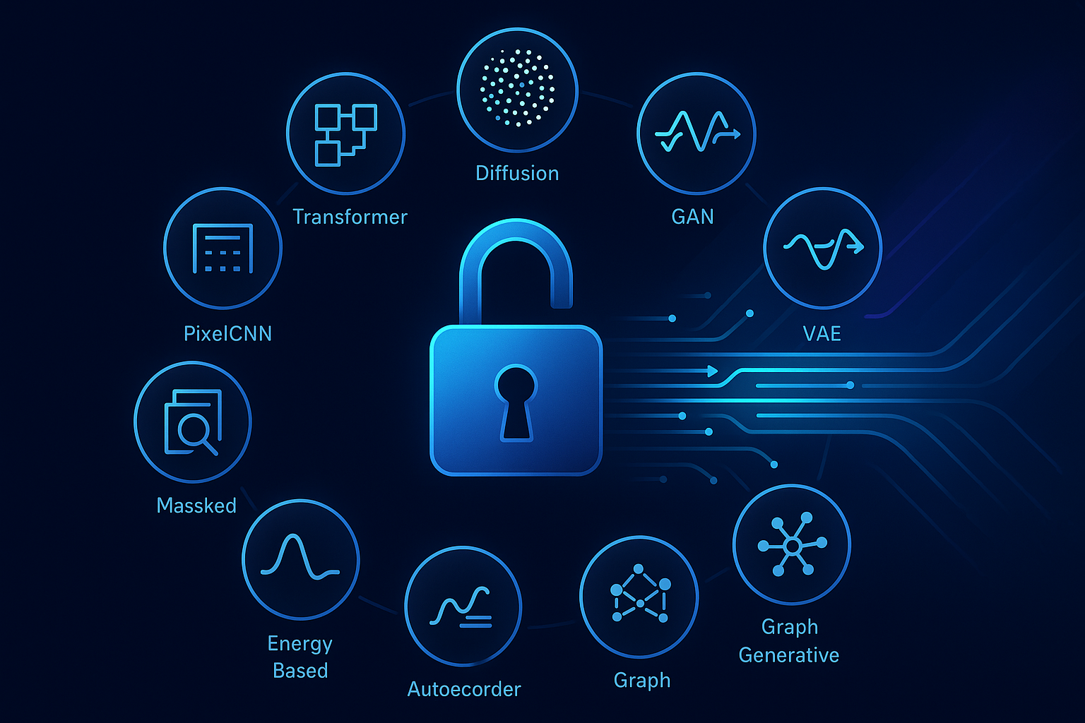
If data is the new oil, then generative AI is the refinery that turns raw information into usable products: text, images, code, simulations, even new datasets. In this guide, you’ll learn how to unlock the power of data with top generative AI algorithms, when to use each one, how to stand them up quickly, what to watch out for, and how to measure success. It’s written for data leaders, ML engineers, analysts, and product teams who want practical, step-by-step instructions—without the math-heavy detours.
Key takeaways
- Match the method to the job. Autoregressive models excel at text and code, diffusion at images and multimodal, flows at exact likelihoods, and VAEs at controllable latent spaces.
- Data quality beats parameter counts. Curate, de-duplicate, and align to tasks before you scale.
- Evaluate with the right metric. Use perplexity or task accuracy for language, FID/IS for images, NLL for likelihood models, BLEU/ROUGE/BERTScore for generation quality.
- Safety isn’t optional. Guardrails (filtering, retrieval grounding, constrained decoding, DP-SGD) prevent costly failures.
- Ship in weeks, not years. Start small, automate evaluation, and expand with retrieval, conditioning, and feedback loops.
1) Autoregressive Transformers (Large Language Models)
What it is & benefits
Autoregressive Transformers predict the next token given previous tokens. They’re the foundation for modern text, code, and multimodal generation. Benefits include strong few-shot behavior, composability with tools (retrieval, function calling), and straightforward scaling.
Prerequisites
- Skills: Python, deep learning basics.
- Stack: PyTorch or JAX/TF; accelerator (A10/A100 or comparable), or managed endpoints.
- Data: Domain text/code, cleaned and filtered.
- Low-cost alternative: Fine-tune a small open model or use LoRA/QLoRA on a single GPU.
Step-by-step (beginner)
- Start with a pre-trained base (small to medium).
- Prepare a curated corpus: remove PII, duplicates, and near-duplicates; add task exemplars.
- Fine-tune with causal LM objective; monitor validation loss and perplexity.
- Add instruction tuning data for helpfulness and formatting.
- Deploy with nucleus sampling (p) and temperature; log prompts/outputs (with privacy).
Beginner modifications & progressions
- Easier: Prompt-only few-shot; no training.
- Harder: Multi-task SFT + preference optimization; add tool use and retrieval.
Recommended cadence & metrics
- Cadence: Re-train or refresh adapters monthly or when data drifts.
- Metrics: Perplexity for base modeling; task-specific accuracy; BLEU/ROUGE/BERTScore for generation quality; human eval for sensitive tasks.
Safety & common mistakes
- Mistake: Letting the model “wing it” on facts. Fix with retrieval grounding and constrained decoding (JSON schemas).
- Mistake: Uncatalogued prompts and outputs. Fix with observability and red-teaming datasets.
Mini-plan
- Collect 1–2k domain exemplars.
- LoRA-tune a 7–13B model; evaluate with a 200-example holdout.
- Add retrieval for reference answers; ship a pilot.
2) Diffusion Models (Score-based & Latent Diffusion)
What it is & benefits
Diffusion models learn to denoise data, enabling high-fidelity image, audio, and video generation. Latent diffusion moves denoising to a compact latent space, making training and inference dramatically more efficient while preserving quality. Benefits include controllable conditioning (text, masks, depth) and excellent sample quality.
Prerequisites
- Skills: Vision basics, PyTorch, mixed precision.
- Stack: At least one strong GPU; for training from scratch, multiple GPUs.
- Data: Balanced, licensed images/captions; captions can be synthetic.
- Low-cost alternative: Fine-tune a latent diffusion checkpoint with DreamBooth/Textual Inversion or LoRA.
Step-by-step (beginner)
- Choose a latent diffusion backbone with a permissive license.
- Build a small, rights-cleared training set; generate clean captions if needed.
- Fine-tune with classifier-free guidance; validate on a small prompt suite.
- Add conditioning (seg masks, depth) for controllability.
Beginner modifications & progressions
- Easier: Prompt-engineering a pre-trained checkpoint; no training.
- Harder: Train your own autoencoder + text encoder; scale to higher resolution.
Recommended cadence & metrics
- Cadence: Refresh adapters quarterly or when style drifts.
- Metrics: FID and Inception Score for image quality; human pairwise preference; latency/cost.
Safety & common mistakes
- Mistake: Training on unlicensed or biased data. Use only licensed/consented sets and audit class/attribute balance.
- Mistake: Over-guidance causing artifacts; tune guidance scale and steps.
Mini-plan
- Pick 2–3 core use cases (e.g., product renderings).
- Fine-tune a latent diffusion model with 2–5k curated examples.
- Validate with FID and a human rubric; deploy an internal sampler.
3) Generative Adversarial Networks (GANs)
What it is & benefits
GANs pit a generator against a discriminator in a minimax game. They’re fast at inference and can excel at specific domains (faces, textures, data augmentation).
Prerequisites
- Skills: PyTorch, training stability tricks.
- Stack: Single GPU for niche datasets; multi-GPU for high-res.
- Data: Consistent framing and style; hundreds to tens of thousands of samples.
- Low-cost alternative: Fine-tune a lightweight GAN or use diffusion for better stability.
Step-by-step (beginner)
- Start with a stable GAN architecture (e.g., modern variants with gradient penalties).
- Balance G/D learning rates; use spectral norm/regularization.
- Track FID/IS on a fixed validation set; stop early if mode collapse signs appear.
Beginner modifications & progressions
- Easier: Use a pre-trained GAN and fine-tune on your style.
- Harder: Add conditioning (labels, text) and progressive growing or style blocks.
Recommended cadence & metrics
- Cadence: Retrain when target style or dataset shifts.
- Metrics: FID/IS; diversity measures; downstream performance if used for augmentation.
Safety & common mistakes
- Mistake: Mode collapse. Use mini-batch discrimination, gradient penalties, or TTUR scheduling.
- Mistake: Overfitting small datasets. Use augmentation and early stopping.
Mini-plan
- Assemble 5k consistent images.
- Train a conditional GAN with augmentation and TTUR.
- Review FID trajectory; select best checkpoint by validation FID.
4) Variational Autoencoders (VAEs)
What it is & benefits
VAEs learn a latent representation with a regularized posterior so you can sample, interpolate, and control outputs via latent arithmetic. They’re robust, interpretable, and great for anomaly detection and controllable generation.
Prerequisites
- Skills: Autoencoders, KL divergence intuition.
- Stack: Single GPU is fine for modest resolution.
- Data: Clean and representative; augment for robustness.
- Low-cost alternative: Use a pre-trained VAE encoder/decoder (often bundled with latent diffusion).
Step-by-step (beginner)
- Start with a β-VAE; tune β to trade off reconstruction vs. disentanglement.
- Train on reconstructions; validate with MSE/PSNR/SSIM.
- Sample from the prior and inspect for plausibility; adjust capacity or β.
Beginner modifications & progressions
- Easier: Plain autoencoder for reconstruction only.
- Harder: Hierarchical VAEs and vector-quantized latents for crispness.
Recommended cadence & metrics
- Cadence: Refresh quarterly.
- Metrics: Reconstruction error; FID for samples; latent traversals for interpretability.
Safety & common mistakes
- Mistake: Posterior collapse. Use KL annealing, skip connections, or capacity scheduling.
- Mistake: Unchecked latent drift. Constrain or regularize latent priors.
Mini-plan
- Train a β-VAE on domain images.
- Map samples into latent space; visualize 2D UMAP.
- Build a slider UI for controllable synthesis.
5) Normalizing Flows (NICE, RealNVP, Glow)
What it is & benefits
Flows are invertible networks with tractable log-likelihoods. You get exact density estimation, exact sampling, and interpretable latents—ideal when likelihoods matter (compression, out-of-distribution detection, scientific modeling).
Prerequisites
- Skills: Change-of-variables formula; coupling layers.
- Stack: Single to few GPUs depending on resolution.
- Data: Continuous, normalized; sometimes dequantized.
Step-by-step (beginner)
- Start with RealNVP-style affine coupling; add permutations/1×1 invertible convs.
- Train by maximizing log-likelihood; monitor NLL on validation data.
- Sample and sanity-check; add depth/capacity if underfitting.
Beginner modifications & progressions
- Easier: Low-dimensional tabular flows.
- Harder: High-res images with Glow-style architectures.
Recommended cadence & metrics
- Cadence: Retrain when data distribution shifts.
- Metrics: NLL (bits-per-dimension), OOD detection rates.
Safety & common mistakes
- Mistake: Ignoring dequantization for discrete pixels—produces artifacts.
- Mistake: Overfitting with too-powerful invertible layers; watch validation NLL.
Mini-plan
- Fit a RealNVP to tabular KPIs for density and anomaly scoring.
- Calibrate threshold from validation tails.
- Integrate scores into monitoring dashboards.
6) Autoregressive Image Models (PixelRNN/PixelCNN)
What it is & benefits
These models factorize images pixel-by-pixel or block-by-block, optimizing exact likelihood and capturing fine local structure. Great for research, compression-oriented use, and small images; also useful as teacher models.
Prerequisites
- Skills: CNNs/RNNs; masked convolutions.
- Stack: Single/multi-GPU depending on size.
- Data: Preprocessed, often small (e.g., 32×32 to 128×128).
Step-by-step (beginner)
- Choose a masked CNN implementation.
- Train with cross-entropy per pixel; monitor NLL (bits-per-dim).
- Generate images via ancestral sampling; cache for speed.
Beginner modifications & progressions
- Easier: Tiny datasets (CIFAR-10) to learn the ropes.
- Harder: Conditional variants with labels or text.
Recommended cadence & metrics
- Cadence: Retrain when conditional distribution changes.
- Metrics: NLL; visual crispness; decoding latency.
Safety & common mistakes
- Mistake: Underestimating sampling cost; batch sampling or distillation helps.
- Mistake: Overfitting on tiny datasets; add augmentation.
Mini-plan
- Train a PixelCNN for a brand icon set at 64×64.
- Condition on color palette.
- Export a sampler for design teams.
7) Masked Autoencoders & Masked Language/Image Modeling
What it is & benefits
Masked modeling randomly hides tokens or patches and trains a model to reconstruct them. It’s efficient self-supervision for language and vision, delivering strong representations with less compute—great for pretraining and domain adaptation.
Prerequisites
- Skills: Transformers and tokenization/patching.
- Stack: Single GPU for small configs.
- Data: Unlabeled text or images; masking ratio tuning.
Step-by-step (beginner)
- For text, pretrain with masked token prediction; for images, adopt an asymmetric encoder-decoder with high mask ratio.
- Fine-tune on downstream tasks (classification, QA, detection).
- For generative outputs, couple with a decoder or diffusion stage.
Beginner modifications & progressions
- Easier: Use pre-trained masked encoders; just fine-tune heads.
- Harder: Scale masking schedules and augmentations; combine with contrastive learning.
Recommended cadence & metrics
- Cadence: Re-pretrain quarterly as domain data grows.
- Metrics: Downstream accuracy; zero-shot retrieval; linear probe performance.
Safety & common mistakes
- Mistake: Over-masking that derails learning; start near recommended ratios.
- Mistake: Using masked encoders directly for free-form generation—attach a generative head.
Mini-plan
- Pretrain a masked image encoder on product imagery.
- Fine-tune for defect detection.
- Add a diffusion head for controlled inpainting.
8) Retrieval-Augmented Generation (RAG)
What it is & benefits
RAG pairs a generator with a retriever and a document index, grounding outputs in fresh, verifiable knowledge. Benefits include higher factuality, provenance, and quick updates without re-training the base model.
Prerequisites
- Skills: Vector databases, embedding models, prompt engineering.
- Stack: LLM endpoint, vector store, ingestion pipeline.
- Data: Clean documents with metadata and access control.
Step-by-step (beginner)
- Ingest documents; split into passages; compute embeddings; store in a vector DB.
- On query, retrieve top-k passages; compose a prompt with citations.
- Generate an answer conditioned on retrieved text; log failures and add feedback data.
Beginner modifications & progressions
- Easier: Naive BM25 retrieval as a baseline.
- Harder: Hybrid retrieval, re-ranking, multi-hop, query rewriting, and active learning.
Recommended cadence & metrics
- Cadence: Incremental re-indexing daily; embed new docs on arrival.
- Metrics: Groundedness scores, citation accuracy, answer correctness with human checks.
Safety & common mistakes
- Mistake: Poor chunking/metadata; leads to wrong retrieval.
- Mistake: Ignoring access controls; ensure per-user filtering before generation.
Mini-plan
- Index policy docs and knowledge base.
- Build a retrieval template with explicit citation slots.
- Track groundedness and escalate uncertain answers.
9) Energy-Based Models (EBMs)
What it is & benefits
EBMs learn an energy landscape where data has low energy and non-data has high energy. They’re flexible, support implicit generation (via sampling), and can model complex dependencies.
Prerequisites
- Skills: MCMC or score-matching; stability tricks.
- Stack: Moderate GPUs; patience for sampling.
- Data: Carefully normalized; good negative sampling strategy.
Step-by-step (beginner)
- Choose a training method: score matching, noise-contrastive estimation, or MCMC-based maximum likelihood.
- Train with short-run sampling; add regularization for stability.
- Generate via Langevin dynamics; evaluate with downstream tasks or visual quality.
Beginner modifications & progressions
- Easier: Start with low-dimensional or tabular EBMs.
- Harder: Combine with diffusion or transformers for hybrid models.
Recommended cadence & metrics
- Cadence: Retrain with distribution shifts; cache samples.
- Metrics: Downstream accuracy, EBM calibration, sample diversity.
Safety & common mistakes
- Mistake: Unstable training without proper noise schedules.
- Mistake: Underestimating sampling cost; consider short-run or amortized inference.
Mini-plan
- Train an EBM for anomaly detection in sensor data.
- Use score-based training; set thresholds from validation tails.
- Alert when energy crosses calibrated limits.
10) Graph Generative Models
What it is & benefits
Graph generators create realistic networks—useful in drug discovery, recommender simulations, fraud networks, and logistics. Autoregressive graph models scale to larger graphs and capture structural patterns.
Prerequisites
- Skills: Graph data structures, PyTorch Geometric/DGL.
- Stack: Single GPU for small graphs; more for molecules or large networks.
- Data: Graph datasets with node/edge attributes; canonical ordering or sequence scheme.
Step-by-step (beginner)
- Choose an autoregressive node-and-edge generator or a VAE-style graph model.
- Train on representative graphs; monitor degree distributions and motif statistics.
- Generate graphs; evaluate with MMD and domain constraints (e.g., valency for molecules).
Beginner modifications & progressions
- Easier: Tiny motif libraries to sanity-check.
- Harder: Conditional generation (targets, constraints), reinforcement for validity.
Recommended cadence & metrics
- Cadence: Retrain when topology or schema changes.
- Metrics: MMD over graph statistics; validity/uniqueness/novelty.
Safety & common mistakes
- Mistake: Ignoring domain constraints, producing invalid graphs.
- Mistake: Overfitting to a single topology; diversify training sets.
Mini-plan
- Collect historical transaction graphs.
- Train a graph generator conditioned on customer segments.
- Simulate interventions; measure lift via A/B in a sandbox.
Quick-Start Checklist
- Define a single business use case and target metric.
- Pick the algorithm family that matches the output and constraints.
- Secure licensed, de-duplicated data with metadata and access control.
- Stand up a baseline (pre-trained or small model) in a sandbox.
- Create a frozen evaluation set with automatic and human metrics.
- Add guardrails: retrieval for facts, constrained decoding, content filters, privacy checks.
- Instrument observability: prompts, outputs, latency, cost, and feedback.
Troubleshooting & Common Pitfalls
- Outputs look great but are wrong. Add retrieval grounding, discourage unsupported claims with system prompts, require citations, and refuse when confidence is low.
- Training is unstable (GANs/EBMs). Lower learning rates; use gradient penalties, spectral norm, or score matching; increase batch size if possible.
- Mode collapse or low diversity. Increase diversity penalties, tweak guidance scales (diffusion), or diversify training data.
- Latency too high. Use smaller models with retrieval, distill to compact students, quantize, or cache partial results.
- Data leakage/PII. Add PII scrubbing, blocklist filters, and differential privacy where feasible; audit logs for sensitive strings.
- Evaluation mismatch. Align metrics to use case; automate regression tests; run periodic human reviews.
How to Measure Progress (by Modality)
- Language & code: Perplexity, task accuracy, BLEU/ROUGE/BERTScore, pass@k (for code), groundedness and citation correctness.
- Images: FID, Inception Score, CLIP-based alignment, expert blind ratings.
- Likelihood models: NLL/bits-per-dimension; OOD detection accuracy.
- Graphs: MMD on degree/triangle/cluster distributions; domain validity rates.
- Business outcomes: Time-to-first-draft, resolution time, conversion rate uplift, cost per request.
A Simple 4-Week Starter Plan
Week 1 — Define & Baseline
- Pick one use case (e.g., support reply drafts or product visuals).
- Prepare a 500–1,000 example eval set with acceptance criteria.
- Stand up a pre-trained model or checkpoint; log metrics.
Week 2 — Data & Guardrails
- Curate/clean fine-tuning data; remove PII and duplicates.
- Add retrieval grounding for factual tasks; design prompts/templates.
- Ship an internal alpha; collect structured feedback.
Week 3 — Fine-Tune & Evaluate
- Fine-tune (LoRA/QLoRA or small diffusion/GAN adapter).
- Run automatic metrics and human review; fix failure modes.
- Add constrained decoding and safety filters.
Week 4 — Harden & Launch
- Optimize latency and cost (quantization, caching).
- Create dashboards for metrics and drift; schedule re-training.
- Launch to a small cohort with rollback plans and feedback forms.
FAQs
1) Which algorithm should I start with if I only have text?
Use an autoregressive Transformer with retrieval-augmented generation. Fine-tune with LoRA on task examples and ground outputs in your knowledge base.
2) How do I prevent hallucinations?
Ground with retrieval, use prompts that require citing sources, set temperature low for factual tasks, and block unsupported claims with validators.
3) Do I need to train diffusion models from scratch?
Usually not. Fine-tuning a latent diffusion model on a curated set yields strong results with a fraction of the compute.
4) Are GANs obsolete?
No. Diffusion leads in generality and stability, but GANs remain useful for fast, domain-specific synthesis and augmentation when you can train them stably.
5) How do I measure image generation quality?
Use FID and Inception Score plus human pairwise ratings and CLIP-based alignment for text-to-image tasks.
6) When do flows beat VAEs or diffusion?
When you need exact likelihoods, calibrated densities, or invertibility—for example in compression, anomaly detection, or scientific modeling.
7) Can masked models generate content directly?
Masked encoders excel at representation learning. For generation, pair them with decoders or a diffusion head, or use autoregressive decoders.
8) What’s the easiest way to add fresh knowledge?
RAG. Index documents, retrieve top-k, and condition the generator. It updates as soon as your index refreshes.
9) How do I keep models private and compliant?
Scrub PII, restrict logs, segment access, and consider DP-SGD for sensitive training. Validate outputs for policy compliance before release.
10) How big should my first model be?
As small as possible to meet acceptance criteria. Start with compact models plus retrieval and scale only if metrics demand it.
11) How often should I retrain?
When data or style drifts, or performance drops below thresholds—often monthly for adapters, quarterly for foundations.
12) What if my evaluations disagree with user satisfaction?
Add human-in-the-loop review, expand metrics (e.g., groundedness, readability), and refine prompts/datasets to reflect real tasks.
Conclusion
Generative AI turns raw data into leverage—drafts into publishable content, pixels into products, graphs into simulations, and logs into insight. By choosing the right algorithm family, grounding it in clean data, evaluating with fit-for-purpose metrics, and adding guardrails, you can move from prototypes to reliable systems quickly and responsibly.
CTA: Pick one use case, choose the matching algorithm from this list, and ship your first grounded, measured generative system in the next four weeks.
References
- “Generative Adversarial Networks,” arXiv, 2014-06-10. https://arxiv.org/abs/1406.2661
- “Auto-Encoding Variational Bayes,” arXiv, 2013-12-20. https://arxiv.org/abs/1312.6114
- “Denoising Diffusion Probabilistic Models,” arXiv, 2020-06-19. https://arxiv.org/abs/2006.11239
- “High-Resolution Image Synthesis with Latent Diffusion Models,” arXiv/CVPR, 2021-12-20. https://arxiv.org/abs/2112.10752
- “Photorealistic Text-to-Image Diffusion Models with Deep Language Understanding,” arXiv, 2022-05-23. https://arxiv.org/abs/2205.11487
- “Attention Is All You Need,” arXiv, 2017-06-12. https://arxiv.org/abs/1706.03762
- “Language Models are Few-Shot Learners,” arXiv/NeurIPS, 2020-05-28. https://arxiv.org/abs/2005.14165
- “Conditional Image Generation with PixelCNN Decoders,” arXiv, 2016-06-16. https://arxiv.org/abs/1606.05328
- “Pixel Recurrent Neural Networks,” arXiv, 2016-01-25. https://arxiv.org/abs/1601.06759
- “Glow: Generative Flow with Invertible 1×1 Convolutions,” arXiv, 2018-07-09. https://arxiv.org/abs/1807.03039
- “NICE: Non-linear Independent Components Estimation,” arXiv, 2014-10-30. https://arxiv.org/abs/1410.8516
- “How to Train Your Energy-Based Models,” arXiv, 2021-01-09. https://arxiv.org/abs/2101.03288
- “Retrieval-Augmented Generation for Knowledge-Intensive NLP Tasks,” arXiv, 2020-05-22. https://arxiv.org/abs/2005.11401
- “GANs Trained by a Two Time-Scale Update Rule Converge to a Local Nash Equilibrium (introducing FID),” arXiv, 2017-06-26. https://arxiv.org/abs/1706.08500
- “Improved Techniques for Training GANs (introducing Inception Score),” arXiv, 2016-06-10. https://arxiv.org/abs/1606.03498
- “BLEU: a Method for Automatic Evaluation of Machine Translation,” ACL Anthology, 2002-07. https://aclanthology.org/P02-1040.pdf
- “ROUGE: A Package for Automatic Evaluation of Summaries,” ACL Anthology, 2004-07. https://aclanthology.org/W04-1013/
- “BERTScore: Evaluating Text Generation with BERT,” arXiv, 2019-04-21. https://arxiv.org/abs/1904.09675
- “Deep Learning with Differential Privacy,” arXiv, 2016-07-01. https://arxiv.org/abs/1607.00133
