Continual Learning: Strategies to Combat Catastrophic Forgetting

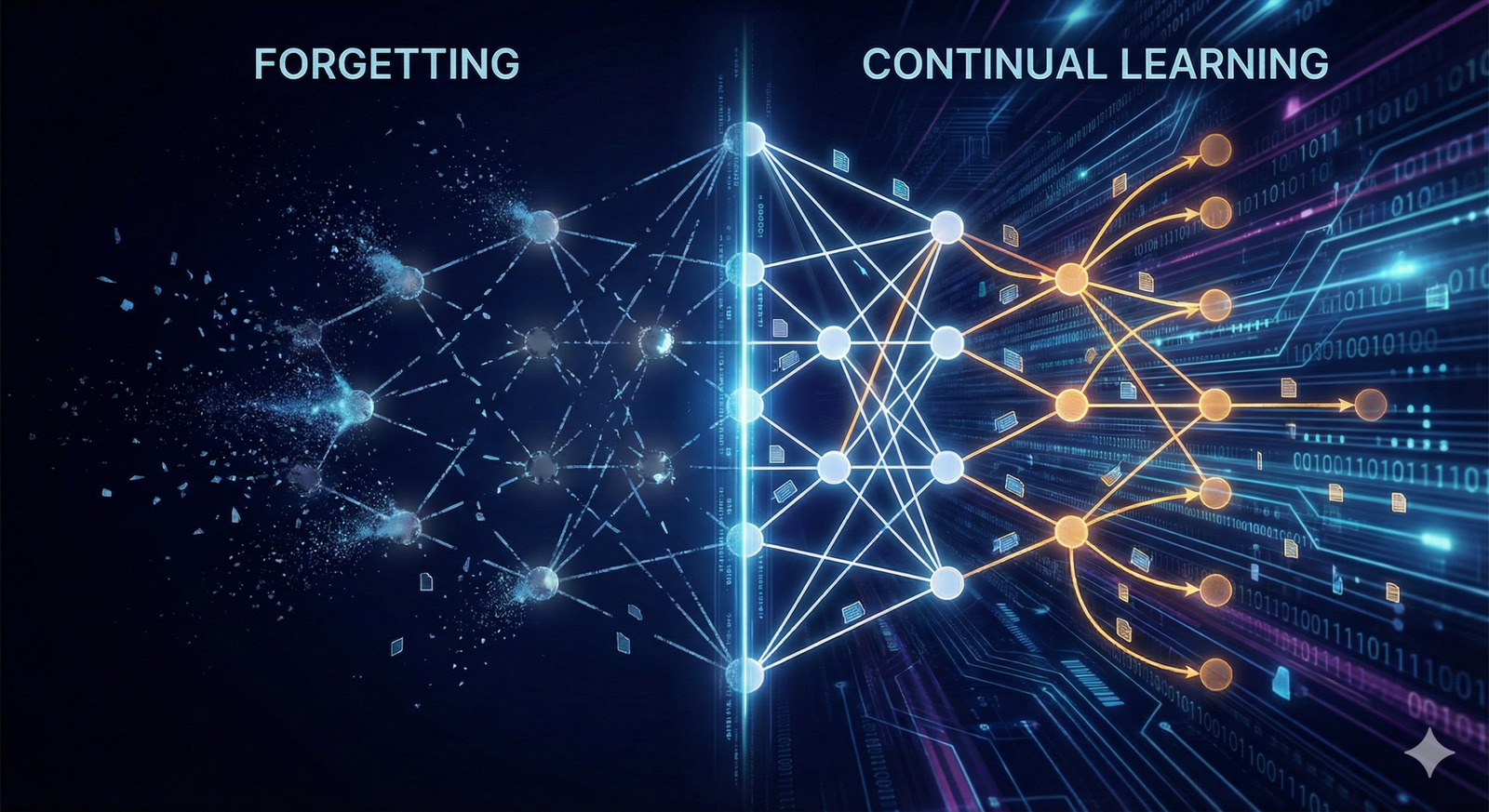
Imagine learning to drive a car and, in the process, completely forgetting how to ride a bicycle. For humans, this scenario sounds absurd. Our brains are capable of lifelong learning, acquiring new skills and memories while retaining old ones. We adapt to new environments without erasing our past experiences. However, for standard artificial neural networks, this erasure is the default behavior. This phenomenon, known as catastrophic forgetting, remains one of the most significant hurdles in the development of truly intelligent, adaptable AI systems.

Continual learning (CL)—also referred to as lifelong learning or incremental learning—is the field of machine learning dedicated to solving this problem. It seeks to create algorithms and architectures that can learn sequentially, accumulating knowledge over time just as humans do. As artificial intelligence moves from static, pre-trained models to dynamic agents that must operate in changing real-world environments, continual learning has become a critical area of research and development.

In this comprehensive guide, we will explore the mechanisms behind catastrophic forgetting, the core strategies used to achieve continual learning, and the practical frameworks that developers and researchers are using to build more resilient AI systems.

Key Takeaways

• Catastrophic forgetting occurs when a neural network overwrites the weights optimized for a previous task while learning a new one, leading to a drastic drop in performance on the old task.
• Continual learning aims to balance the stability-plasticity dilemma: maintaining stability to preserve old knowledge while remaining plastic enough to learn new information.
• Three main approaches dominate the field: regularization-based methods (constraining weight updates), replay-based methods (revisiting old data), and architecture-based methods (expanding the network).
• Evaluation is complex, requiring metrics not just for accuracy on the current task, but also for backward transfer (retention) and forward transfer (accelerated learning of new tasks).
• Real-world applications range from robotics and autonomous vehicles to personalized digital assistants that evolve with the user.

Who This Is For (And Who It Isn’t)

This guide is designed for data scientists, machine learning engineers, AI researchers, and technical product managers who want a deep understanding of how to build models that adapt over time.

• It is for you if: You are familiar with the basics of deep learning and neural networks and want to understand how to train models on streaming data or sequential tasks.
• It is not for you if: You are looking for a non-technical, high-level overview of general AI buzzwords, or if you are looking for a basic “What is AI?” tutorial. We assume some familiarity with concepts like loss functions, weights, and backpropagation.

The Core Problem: Understanding Catastrophic Forgetting

To understand the solution, we must first deeply understand the problem. In standard supervised learning, a model is trained on a fixed dataset where all data is available at once (i.i.d. assumption—independent and identically distributed). The optimization algorithm, such as Stochastic Gradient Descent (SGD), adjusts the network’s weights to minimize the error across this entire dataset.

However, the real world is rarely static. Data often arrives in streams, or tasks change over time. When a neural network trained on Task A is subsequently trained on Task B, the backpropagation algorithm adjusts the weights to minimize the error for Task B. Since the data for Task A is no longer present during this update, the gradients have no incentive to preserve the configurations that were useful for Task A. The result is that the weights are aggressively overwritten.

This isn’t a gradual degradation; it is often “catastrophic.” A model that achieved 99% accuracy on digit recognition might drop to near-random guessing on digits after being trained to recognize letters.

The Stability-Plasticity Dilemma

At the heart of catastrophic forgetting lies the stability-plasticity dilemma, a fundamental constraint in both biological and artificial neural systems.

• Plasticity refers to the ability of the system to integrate new knowledge. A highly plastic system learns quickly and adapts easily to new data.
• Stability refers to the ability to retain previously acquired knowledge. A stable system is resistant to disruption.

Standard neural networks are typically highly plastic but lack stability mechanisms. Conversely, if we freeze the weights of a network to preserve old memories (high stability), we prevent it from learning anything new (zero plasticity). Continual learning seeks to find the optimal trade-off or a mechanism to bypass this trade-off entirely.

Defining Continual Learning

Continual learning is the paradigm where an algorithm learns from a stream of data, with the goal of preserving performance on past tasks while mastering new ones. Unlike transfer learning, where the goal is usually to perform well on the target (new) task potentially at the expense of the source (old) task, continual learning treats all tasks—past and present—as equally important.

The Three Scenarios of Continual Learning

In the academic literature and practical application, CL is often categorized into three distinct scenarios based on the availability of task identity during training and inference:

1. Task-Incremental Learning: The model is told which task it is performing. For example, a robot is explicitly told, “Now you are playing tennis,” or “Now you are cooking.” The model can use task-specific modules or heads. This is the easiest scenario.
2. Domain-Incremental Learning: The task structure remains the same, but the input distribution changes. An example is an autonomous car trained in sunny California that must now learn to drive in snowy Norway. The “task” (driving) is the same, but the “domain” (environment) is radically different.
3. Class-Incremental Learning: The model must learn to recognize new classes of objects over time and, crucially, must be able to distinguish between all classes (past and present) without being told which task the current input belongs to. This is the hardest and most realistic scenario for general AI.

Core Approaches to Continual Learning

Researchers have developed three primary families of strategies to enable machine learning plasticity while preventing catastrophic forgetting. In practice, the best systems often combine elements from multiple families.

1. Regularization-Based Methods

Regularization approaches attempt to solve the problem by imposing constraints on the weight updates of the neural network. The logic is simple: if a specific neuron or connection was crucial for solving Task A, we should prevent it from changing too much when we learn Task B.

Elastic Weight Consolidation (EWC)

One of the most famous algorithms in this category is Elastic Weight Consolidation (EWC). EWC draws inspiration from synaptic consolidation in the brain. It estimates the “importance” of each parameter (weight) for the previous tasks.

• How it works: After training on Task A, EWC calculates the Fisher Information Matrix to approximate the importance of each weight. Weights that are critical for Task A are assigned a high importance value.
• The constraint: When training on Task B, a penalty term is added to the loss function. This quadratic penalty discourages changes to the weights that have high importance scores. Unimportant weights are left free to change (high plasticity), while important weights are “elastic” but resistant to change (high stability).
• Pros: Requires no storage of old data; computationally efficient during inference.
• Cons: Can be computationally expensive to calculate the Fisher matrix; performance degrades as the number of tasks becomes very large because the weights become too constrained (too rigid).

Synaptic Intelligence (SI)

Similar to EWC, Synaptic Intelligence tracks the importance of weights during training. It accumulates the contribution of each parameter to the reduction of the loss function over the training trajectory. This allows the model to estimate importance online, without needing a separate post-training calculation step like EWC.

Learning Without Forgetting (LwF)

Learning Without Forgetting uses knowledge distillation. Before training on the new task, the current network generates predictions (soft targets) for the new data. During training, the network is optimized to minimize the loss on the new ground-truth labels and to match the predictions of the “old” network on the new data. This preserves the input-output mapping of the previous state without needing to access the old data or calculate weight importance explicitly.

2. Replay-Based Methods (Memory)

Replay-based methods are widely considered the most effective strategy for difficult scenarios like Class-Incremental Learning. They work by re-training the model on a mix of new data and a small subset of old data.

Experience Replay

This is the most straightforward approach. The system maintains a replay buffer—a small, fixed-size memory bank that stores a few representative examples from previous tasks.

• How it works: When training on Task B, the model samples a mini-batch from the new Task B data and mixes it with a mini-batch sampled from the replay buffer (Task A data). The model essentially “rehearses” the old tasks interleaved with the new one.
• Challenges: The main challenge is selecting which examples to store. Random sampling is a baseline, but more sophisticated methods (“herding”) try to select examples that best approximate the geometric center or the boundaries of the old data distribution.

Generative Replay

Storing raw data raises privacy concerns (e.g., in healthcare or finance) and memory constraints. Generative Replay solves this by training a separate generative model (like a GAN or VAE) alongside the classifier.

• How it works: Instead of storing images of Task A, the system trains a generator to produce images that look like Task A. When training on Task B, the generator creates “pseudo-data” representing Task A, which is mixed with the real Task B data.
• The “Dreaming” Analogy: This is often compared to human dreaming, where the brain consolidates memories by replaying neural patterns during sleep.

Gradient Episodic Memory (GEM)

GEM and its efficient variant (A-GEM) use the replay buffer differently. Instead of just mixing data, they use the stored examples to constrain the gradients. When the model computes a gradient update for the new task, GEM checks if this update would increase the loss on the stored examples. If it does (implying forgetting), the gradient is projected (rotated) so that it minimizes the new task loss without harming the old task performance.

3. Architecture-Based Methods

Architecture-based methods (or parameter isolation methods) tackle the problem by modifying the structure of the neural network itself. They dedicate different subsets of the network parameters to different tasks.

Parameter Isolation

In this approach, the network masks out certain neurons for specific tasks. For Task A, specific pathways are activated. For Task B, different pathways are used.

• Fixed Network: Some methods attempt to find “sub-networks” within a fixed large model (e.g., PackNet).
• Pros: Can achieve zero forgetting because the weights for Task A are completely frozen/masked during Task B training.
• Cons: Capacity saturation. Eventually, you run out of free neurons in a fixed network.

Dynamic Expansion (Progressive Neural Networks)

If a fixed network fills up, why not grow it? Progressive Neural Networks instantiate a new column of neurons for every new task. The new column is trained on the new task but receives lateral connections from the frozen columns of previous tasks.

• Pros: Guarantees no catastrophic forgetting; allows transfer of knowledge via lateral connections.
• Cons: The model size grows linearly with the number of tasks. This is not sustainable for lifelong learning with hundreds of tasks, but effective for smaller sequences.

Deep Dive: The Role of Representations in Retention

Recent research has shifted focus from just preserving weights to preserving representations. Deep learning memory is not just about specific numbers in a matrix; it is about the geometric relationships in the latent space.

When a model experiences catastrophic forgetting, the feature extractor (the early layers of the network) often rotates or distorts the latent space to accommodate the new class. This distortion ruins the boundaries established for the old classes.

Self-supervised learning is emerging as a powerful ally here. By pre-training models on vast amounts of unlabeled data, models learn robust, generalizable feature representations that are less likely to change drastically when fine-tuned on specific sequential tasks. This “robust backbone” acts as a stabilizing anchor, reducing the severity of forgetting even before specific CL algorithms are applied.

Evaluating Performance: Beyond Accuracy

In standard machine learning, we look at the test accuracy. In continual learning, a single number is insufficient. To properly evaluate a CL system, we must look at three dimensions:

1. Average Accuracy: The average performance across all tasks learned so far.
2. Backward Transfer (BWT): This measures the influence of learning a new task on the performance of old tasks.
   • Negative BWT: Catastrophic forgetting (learning Task B hurt Task A).
   • Positive BWT: The Holy Grail. Learning Task B actually improved Task A (e.g., learning to recognize “trucks” helped the model better understand “cars” because it learned better edge detection).
3. Forward Transfer (FWT): This measures the zero-shot performance on a new task before training on it, based on what the model already knows. Does knowing Task A make it easier/faster to learn Task B?
4. Memory Size: How many parameters or bytes of storage (replay buffer) does the method require? A method that stores all previous data is not a continual learner; it’s just a retrained batch learner.
5. Computational Cost: How much compute is required to update the model? Does it need to re-process extensive data?

Real-World Applications of Continual Learning

While much of CL research is academic, industrial applications are rapidly maturing as of 2026.

1. Robotics and Autonomous Systems

A home robot deployed in Japan encounters different objects, layouts, and cultural norms than one deployed in the US. Furthermore, the robot’s environment changes: families buy new furniture, get pets, or have children. An autonomous agent must learn to recognize these new elements (a new sofa, a new obstacle) without forgetting how to navigate the hallway or recognize the owner. Continual learning allows robots to adapt “on the edge” without needing constant re-training from a central server.

2. Personalized Digital Assistants

Current LLMs (Large Language Models) are generally static snapshots of the internet from their training date. A true personal assistant needs to learn you. If you tell it “I’m vegan” today, and “I hate cilantro” next month, it must accumulate these preferences. Standard fine-tuning might cause it to forget general knowledge (like how to write a poem). Continual learning enables personalization that accumulates context over years of interaction.

3. Pharmaceutical Drug Discovery

In drug discovery, models are trained to predict the properties of molecules. As new experimental data becomes available (which is expensive and slow), the model should update its understanding. Retraining from scratch on the massive historical database every time a new batch of experiments is run is computationally prohibitive. CL allows the model to ingest the new lab results incrementally.

4. Financial Fraud Detection

Fraud patterns are adversarial; they evolve constantly to bypass detection. A model trained on 2020 fraud patterns will fail in 2026. However, old types of fraud don’t disappear—they just become less frequent. A CL system adapts to the new attack vector while retaining the ability to catch the classic “Nigerian Prince” scam, ensuring comprehensive security coverage.

Common Challenges and Pitfalls

Implementing continual learning is not as simple as importing a library. Here are the practical pitfalls engineers face.

The “Capacity Gap”

Even with perfect regularization, a fixed-size neural network has a finite capacity. It cannot learn an infinite number of tasks. Eventually, the stability-plasticity trade-off hits a wall where the model is saturated.

• Solution: Use dynamic architectures or periodic “distillation” cycles where the model is pruned and compressed to free up capacity.

Replay Buffer Bias

If you use Experience Replay, the small buffer can become biased. If you store 100 images of “cars” but the real world distribution was 90% sedans and 10% trucks, your buffer might accidentally capture only sedans. Over time, the model’s “memory” of cars becomes skewed, leading to drift in concept definitions.

• Solution: Use “Herding” or “Core-set selection” strategies to ensure the buffer mathematically represents the distribution of the original data.

Hyperparameter Sensitivity

Regularization methods like EWC are notoriously sensitive to the regularization coefficient (lambda). Set it too high, and the model learns nothing new. Set it too low, and it forgets everything. This hyperparameter often needs to be tuned per task, which defeats the purpose of autonomous continual learning.

• Solution: Use adaptive methods that automatically scale the regularization strength based on the gradient magnitude.

Tools and Frameworks for Continual Learning

For practitioners looking to implement these strategies, several open-source libraries have standardized the benchmarks and algorithms.

1. Avalanche: Maintained by the ContinualAI non-profit, this is currently one of the most comprehensive libraries (based on PyTorch). It provides benchmarks (Split-MNIST, CIFAR-100, CORe50), strategies (EWC, LwF, GEM, Replay), and metrics out of the box.
2. Sequoia: A research library focused on bridging the gap between continual learning and reinforcement learning.
3. Mammoth: A lightweight library specifically designed for efficient replay-based methods and managing buffer strategies.
4. Renate: A library often used for automatic retraining of neural networks, providing robust implementations of continual learning algorithms for tabular and image data.

Future Trends: Where is CL Heading?

As we look toward the latter half of the 2020s, continual learning is intersecting with other frontier AI disciplines.

Neuromorphic Computing

Traditional hardware (GPUs) separates memory and processing. The brain integrates them. Neuromorphic chips (like Intel’s Loihi or IBM’s NorthPole) mimic biological neurons and synapses. These chips are naturally suited for continual learning because they support local, incremental plasticity—updating specific “synapses” on the chip without needing to retrieve global data from RAM.

Meta-Continual Learning (Learning to Learn Continually)

Instead of hand-crafting the rules for EWC or Replay, researchers are using meta-learning to learn the learning rule. The model is trained on a variety of sequential tasks, and the objective is to optimize its own weight-update mechanism so that future sequential learning creates minimal interference. This is “AI designing AI,” specifically for retention.

System-Level Solutions (RAG + CL)

For Large Language Models, the industry is currently favoring a hybrid approach. Instead of updating the model weights (which is risky and expensive), they use Retrieval-Augmented Generation (RAG) as a form of non-parametric memory. The “continual learning” happens in the vector database (adding new documents), while the frozen LLM reasons over them. However, true CL is still needed to update the reasoning capabilities of the model, not just its knowledge base.

Conclusion

Combating catastrophic forgetting is one of the grand challenges of artificial intelligence. It is the barrier standing between narrow, static tools and true lifelong learning agents. While no “silver bullet” algorithm exists yet, the combination of replay buffers, regularization, and dynamic architectures allows us to build systems that are significantly more robust than they were just a few years ago.

For developers and organizations, the shift to continual learning requires a mindset shift: from “train once, deploy forever” to “deploy, monitor, and learn continually.” By respecting the stability-plasticity dilemma and implementing the strategies outlined above, we can create AI that grows with us, remembering the past while mastering the future.

Next Steps

If you are ready to implement continual learning in your projects:

1. Audit your data streams: Is your data i.i.d. or sequential? If sequential, you have a CL problem.
2. Start with Replay: If privacy and memory allow, Experience Replay is the most robust baseline.
3. Download Avalanche: Use the Avalanche library to benchmark a simple EWC or Replay model against a standard fine-tuning loop on your specific data to quantify the severity of forgetting in your domain.

FAQs

Q: Is continual learning the same as transfer learning? No. Transfer learning focuses on using knowledge from a source task to improve performance on a target task, often ignoring whether the source task is forgotten. Continual learning focuses on learning the target task while preserving performance on the source task.

Q: Can we just retrain the model on all data every time? Technically, yes, and this is often the “upper bound” or gold standard for performance. However, as datasets grow to terabytes or petabytes, retraining from scratch becomes computationally impossible, too slow, or violates data retention policies (e.g., privacy laws requiring data deletion).

Q: Does catastrophic forgetting happen in Large Language Models (LLMs)? Yes. If you fine-tune a generic LLM heavily on medical data, it may lose its ability to generate code or write poetry. This is why techniques like LoRA (Low-Rank Adaptation) and Mix-training (mixing a small amount of pre-training data during fine-tuning) are used to mitigate this.

Q: What is the difference between online learning and continual learning? Online learning refers to processing data one sample (or small batch) at a time because the dataset is too large to fit in memory. Continual learning refers to the distribution shift in that data. You can do online learning on a static distribution without catastrophic forgetting. Continual learning specifically addresses the changing tasks/distributions.

Q: Why don’t humans suffer from catastrophic forgetting? The human brain uses complex mechanisms including dual-memory systems (hippocampus for short-term/fast learning, neocortex for long-term/slow consolidation) and sleep-based consolidation to integrate new memories without erasing old ones. CL methods like Generative Replay are inspired by these biological processes.

Q: What is the “stability-plasticity dilemma”? It is the trade-off where a system must be rigid enough to retain old knowledge (stability) but flexible enough to learn new knowledge (plasticity). Too much stability means no learning; too much plasticity means forgetting.

Q: Are there any industries where continual learning is mandatory? It is critical in edge computing and IoT. Devices like smart thermostats or industrial sensors have limited connectivity and power; they cannot constantly upload data to the cloud for retraining. They must learn and adapt locally on the device, making CL algorithms essential.

Q: Does adding more neurons solve catastrophic forgetting? Not necessarily. In a fully connected network, backpropagation will still alter weights across the entire network to minimize the current loss. Simply adding neurons doesn’t help unless you use an architecture-based CL method (like Progressive Neural Networks) that explicitly isolates or freezes parts of the network.

References

1. Kirkpatrick, J., et al. (2017). “Overcoming catastrophic forgetting in neural networks.” Proceedings of the National Academy of Sciences (PNAS).
2. Parisi, G. I., et al. (2019). “Continual lifelong learning with neural networks: A review.” Neural Networks, Elsevier.
3. De Lange, M., et al. (2021). “A continual learning survey: Defying forgetting in classification tasks.” IEEE Transactions on Pattern Analysis and Machine Intelligence.
4. Hayes, T. L., et al. (2020). “Remind your neural network to prevent catastrophic forgetting.” European Conference on Computer Vision (ECCV).
5. ContinualAI. (2026). “Avalanche: The End-to-End Library for Continual Learning.” Official Documentation. https://avalanche.continualai.org
6. Goodfellow, I., et al. (2013). “An Empirical Investigation of Catastrophic Forgetting in Gradient-Based Neural Networks.” International Conference on Learning Representations (ICLR).
7. Rusu, A. A., et al. (2016). “Progressive Neural Networks.” Google DeepMind.
8. Lopez-Paz, D., & Ranzato, M. (2017). “Gradient Episodic Memory for Continual Learning.” Advances in Neural Information Processing Systems (NeurIPS).
9. Van de Ven, G. M., & Tolias, A. S. (2019). “Three scenarios for continual learning.” arXiv preprint.
10. Thrun, S., & Mitchell, T. M. (1995). “Lifelong Robot Learning.” Robotics and Autonomous Systems.